vtables aren't slow (usually)
A common critique of object-oriented programming - and modern programming more broadly - is its poor “mechanical sympathy”: code structured and executed without consideration for what executes it. Whether this matters to you is its own discussion, but understanding the critique and when it applies is worthwhile. One place to start is with polymorphism.
#include <print>
#include <vector>
#include <memory>

class Animal {
public:
    virtual ~Animal() = default;
    virtual void speak() const = 0;
};

class Dog : public Animal {
public:
    void speak() const override { std::println("woof"); }
};

class Cat : public Animal {
public:
    void speak() const override { std::println("meow"); }

    virtual void other() = 0;
};

void make_noise(Animal** animals, int n) {
    for (int i = 0; i < n; ++i) {
        animals[i]->speak();
    }
}
In the example above, each call to animal->speak() is dispatched at
runtime to a derived class implementation. This is dynamic dispatch (as
opposed to static), and it requires virtual tables for lookup. These
tables live in .rodata and consist of an array of function pointers
(and, unless disabled, some runtime type information). Objects that
inherit from one another extend the base layout, and the vtable follows
the same pattern:
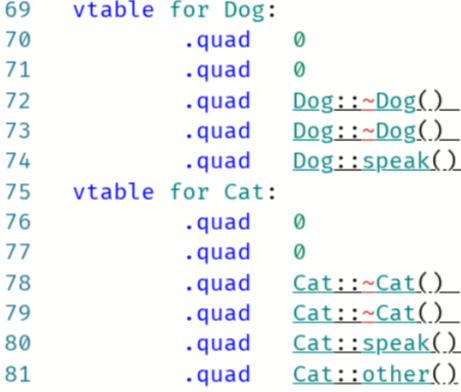
Dog: [vtable*][...Animal...][...Dog...]
Cat: [vtable*][...Animal...][...Cat...]

Dog vtable: [~Dog][Dog::speak]
Cat vtable: [~Cat][Cat::speak][Cat::other]
After compilation with -fno-rtti -O3, this is what we get:
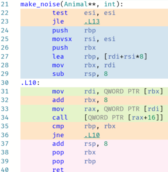
The invocation loads the current Animal*, dereferences the first
element of the derived class instance (its vtable pointer), then calls
the function at speak()’s offset:
.L10:
    mov   rdi, [rbx]  ; load Animal*
    ...
    mov   rax, [rdi]  ; load vtable pointer
    call  [rax+16]    ; call speak() at offset 16
    ...
Assuming these virtual calls are in a hot loop - there’s not really another scenario where this would meaningfully impact performance - a few arguments exist for why this could sometimes be slow.
- CPU backend: the overhead of two dependent loads before the call.
- CPU frontend: the branch predictor can’t anticipate the target.
- Compiler: information is lost that would otherwise be used to optimise.
To put it succinctly, only the third point is likely to matter in practice. The first two seem to apply only when dispatching to functions with trivially small or unrealistically port-saturating bodies, or when array elements are truly random. The former are rarely the target of virtual calls in practice, and may warrant a redesign if they are. The latter is rare, though a solution may be to sort the array by derived class type for batch processing.
The Compiler
So what information is lost, and why does it matter?
An optimising compiler operates on “basic blocks” - regions of code with no branches except at entry and exit. A function may contain several basic blocks, forming a control-flow graph (CFG) where branches are edges between blocks. The whole program, in turn, can be modelled as a call graph of functions which themselves contain control-flow graphs:
 Source: Constructing More Complete Control Flow Graphs Utilizing Directed Gray-Box
Fuzzing
Source: Constructing More Complete Control Flow Graphs Utilizing Directed Gray-Box
Fuzzing
Optimisations happen at three levels: local (within a basic block), global (across a function’s CFG), and interprocedural (across the call graph). These feed into one another and are applied iteratively.
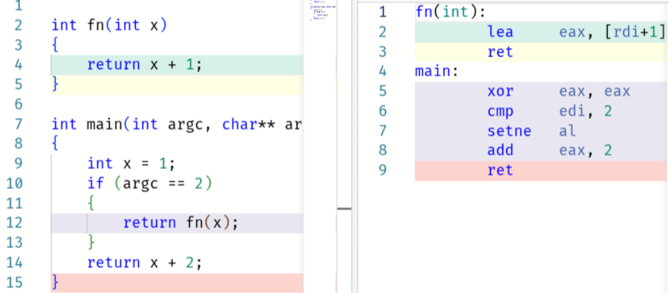
A simple example of an optimisation is constant folding and propagation: arithmetic on compile-time constants is evaluated (“folded”), and the results are “propagated” to dependent variables. For instance:
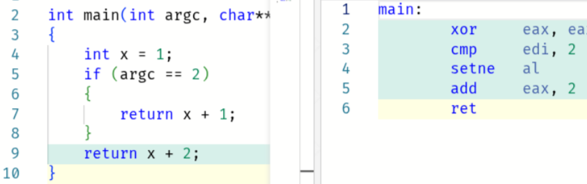
The generated code assumes the return value is 2 (line 7), but if
argc != 2, we add 1 and return 3 (line 9). This required the compiler
to propagate x = 1 to x + 1 = 2 (global) and x + 2 = 3 (local),
then render the function branchless with setne (global).
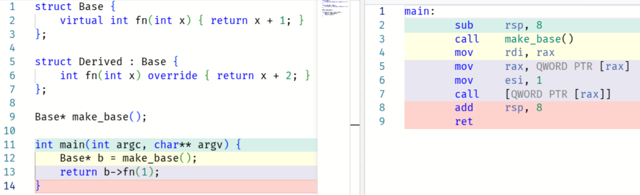
If we move line 7 into it’s own function, the generated code for main
is identical:
Roughly speaking, an interprocedural pass first inlined f(x),
producing an identical main, which was then optimised as above -
globally, locally, and globally again.
The core idea is that these optimisations build on one another. If you
can’t inline f(x), you can’t optimise the caller. This is why virtual
functions can be problematic: the call target is opaque, and the
compiler can’t reason about which implementation will run.
Here, it’s forced to emit the virtual call:
It’s always worth giving the compiler as much information as possible.
One way is through qualifiers like const, noexcept, or final.
Another is simplifying control flow. A third is enabling link-time
optimisation, which addresses the same visibility problem but across
translation units rather than class hierarchies.
The CPU
Before addressing the other two points (extra instructions and branch prediction) some context is useful.
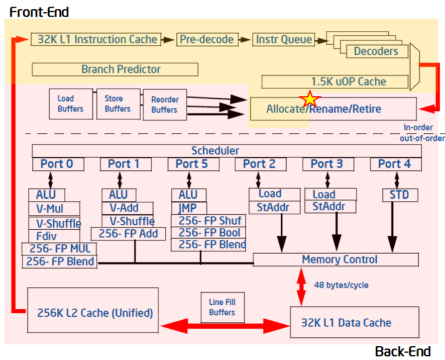
At a high level, the CPU is split into a frontend and backend. The frontend fetches and decodes instructions into micro-ops (uOps). The backend allocates resources to uOps, tracks their dependencies on memory loads or the results of other instructions, and assigns them to execution ports when ready. This diagram from Intel illustrates the split:
 Source:
Top-down Microarchitecture Analysis
Method
Source:
Top-down Microarchitecture Analysis
Method
A cycle where the CPU cannot use a pipeline slot is a stall. If the stall occurs because the frontend couldn’t supply a uOp, it’s frontend-bound. If a uOp was ready but the backend couldn’t execute it, it’s backend-bound.
To recap, the two common arguments for why virtual functions may hurt performance:
- CPU backend: two dependent loads and before the call.
- CPU frontend: the branch predictor can’t anticipate the target.
Backend
The CPU backend uses out-of-order execution. It interprets the stream of uOps from the frontend as a dependency graph rather than a sequence of instructions. Consider this loop summing over an array:
xor eax, eax
.loop:
    add eax, [rdi]
    add rdi, 4
    sub ecx, 1
    jnz .loop
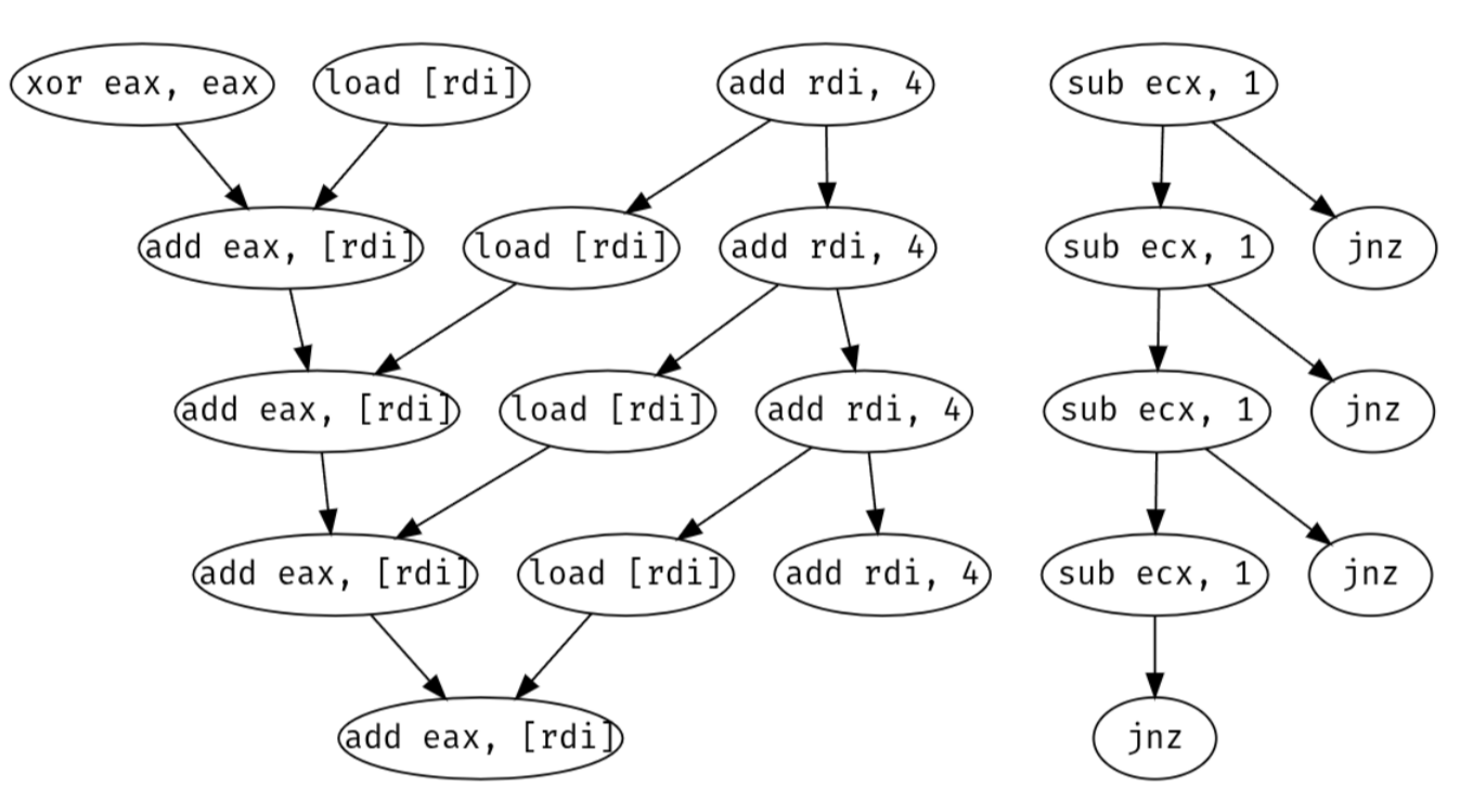
There are two independent dependency chains. The loop counter ecx
depends on its previous value, whereas add eax, [rdi] depends on the
previous eax and the load from [rdi]. The CPU parallelises
horizontally: while waiting on the load, it can perform both adds and
even branch forward to the next iteration.
Assuming sufficient execution ports are available, the bottleneck of a
hot loop is its longest dependency chain. Here, the critical path is the
dependency carried by eax across iterations. If two registers were
used as accumulators and summed at the end, the loop could run up to
twice as fast (assuming the memory subsystem keeps up).
Consider again the earlier loop over Animal**.
.L10:
    mov   rdi, [rbx]  ; load Animal* from array
    mov   rax, [rdi]  ; load vtable pointer
    call  [rax+16]    ; call speak() at offset 16

    add   rbx, 8      ; advance to next pointer
    dec   rcx
    jnz   .L10
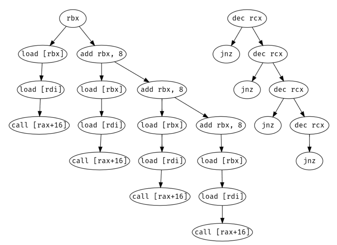
Note that call [rax+16] forms its own dependency graph of all the uOps
involved in executing that function. The backend overlaps these graphs,
running the vtable lookup chain in parallel with whatever work speak()
is doing. Unless speak() is trivially short (nothing to hide the
latency behind) or saturates all execution ports (no spare cycles for
the loads), the vtable overhead effectively disappears.
There’s also the effect on memory. These extra loads require some
bandwidth, but that’s unlikely to matter unless speak() is already
saturating L1. After a few iterations, both the vtables and speak()
instructions for each derived class sit in L1d and L1i respectively. The
only memory overhead from virtual methods is a couple of cache lines for
the tables and bandwidth that probably isn’t being used anyway.
So unless your virtual methods are extremely small, or profiling shows you’re L1-bandwidth-bound or port-saturated, the extra instructions aren’t an issue.
Frontend
To keep the backend fed with uOps, the frontend must speculatively fetch and decode the most probable instructions. This means they are executed but not yet retired to the register file or main memory. If the prediction is wrong, the backend flushes all speculative results while the frontend resteers to the correct branch. This is a branch mispredict, incurring a penalty of roughly as many cycles as there are pipeline stages (~15 on modern CPUs).
Deciding which instructions are “most probable” is the job of the branch predictor. It predicts whether a branch is taken or not-taken, and the target address. The Branch Target Buffer (BTB) caches the destination of each jump as it’s encountered, and the frontend uses those entries to decide what to decode next.
Virtual calls don’t add conditionals - they’re unconditional jumps with several possible targets. Predicting which target to fetch is the job of the Indirect Branch Predictor (IBP). To understand how it works, it helps to first look at taken/not-taken prediction for conditional branches. One method is a 2-bit saturating counter representing four states:
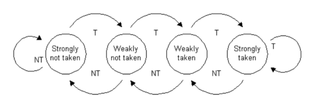 Source: The
microarchitecture of Intel, AMD, and VIA
CPUs
Source: The
microarchitecture of Intel, AMD, and VIA
CPUs
Each time a branch is taken, the state moves in that direction. The frontend predicts whichever direction is the consensus. This works well for branches that don’t change often, but mispredicts 100% of the time for an alternating pattern as the state flips endlessly between the two weak states.
for (int i = 0; i < n; i++)
{
    if (i % 2 == 0)
        action1()
    else
        action2()
}
A solution is to remember the past n directions and maintain 2\^n counters, one for each possible history. In our alternating loop, a single bit of history selects between two counters. Each stays in its strong state, predicting correctly 100% of the time. This is a two-level adaptive predictor:
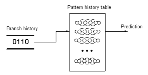 Source: The
microarchitecture of Intel, AMD, and VIA
CPUs
Source: The
microarchitecture of Intel, AMD, and VIA
CPUs
For random data that isn’t 50-50, the two-level predictor performs slightly worse than a single counter, since the history dilutes samples across counters.
Since the CPU can’t store separate histories for every branch, one global table is shared. This predicts the current branch using the previous n outcomes, which works well because future branches often correlate with recent control flow.
A virtual call is an indirect jump, like a switch statement or function pointer, with several possible targets depending on a value in a register or memory. As mentioned, this requires the IBP.
The IBP works similarly to the two-level adaptive predictor, using global branch history to select from the set of predicted targets in the BTB. This works because in practice, control flow often correlates with data.
Animal* a;
if (some_condition) {
    a = new Dog();
} else {
    a = new Cat();
}
a->speak();
In this contrived example, the target is perfectly predicted by the preceding branch. Our loop is harder to reason about as there’s no visible branch history initially:
void make_noise(Animal** animals, int n) {
    for (int i = 0; i < n; ++i) {
        animals[i]->speak();
    }
}
However, the branch history will grow to include branches from previous
iteration speak() calls. The predictor picks up on the relative
ordering of derived classes within animals. So, mispredictions aren’t
likely to be a major issue unless the array’s construction and contents
are truly random.
If your data is random, sort the array by derived class type ahead of
time. The predictor will quickly learn the current speak() target, and
mispredicts will only occur when switching between types.
In practice, the history bits aren’t a literal index into the pattern history table. An index function (similar to a hash) incorporates other information to bias the prediction. The exact index functions and finer details of modern prediction aren’t fully public. Techniques vary; AMD, for instance, has used perceptrons in several microarchitectures.
Summary
Virtual functions are rarely the performance problem they’re made out to be. The compiler’s lost opportunity to inline and optimise is the real cost. The CPU-level concerns (extra loads, branch mispredicts) tend to disappear into the noise unless your virtual methods are trivially small or your data is pathologically random.
Still, understanding why they’re usually fine is more useful than just knowing that they are. The interplay of out-of-order execution, branch prediction, and memory hierarchy explains a lot about where performance does, or doesn’t, come from.